3. Solution Algorithm
3.1. Generation of the initial population
The first step to any Diskpop simulation is the generation of the initial population, based on the initial conditions specified in the parameters.json file.
The input parameters, their meaning and possible values are described in depth in Initial parameters; here, we simply discuss the general workflow that leads to the generation of a population.
Note
When describing the general steps to generate a population, we consider the example of a Monte Carlo-generated population of N = 100 sources, with correlations between the disc properties and the stellar mass. However, we stress that this is not the only possible set up and refero to User interface for more details.
The Young Stellar Objects simulated with Diskpop are composed of a Star and a Disc object, that gets assembled as follows:
- Drawing the stellar masses
The first step to generate a population is determining the values of the stellar masses. In the most realistic case, these are extracted following an Initial Mass Function.
- Assembling the disc
Once the stellar masses are determined, Diskpop moves on to computing the disc parameters - masses, radii, and accretion rates. First, it determines the mean values of each parameter based on the input correlations; then, it draws the actual values from the specified distributions, centered in the just computed mean value and with the specified spread.
The sketch below represents the workflow in the case of the disc mass. The top panel shows a histogram of the stellar masses extracted by the Kroupa (2002) initial mass function; from that, we consider a single value (around 1 \(M_{\odot}\)) marked with a cross. In the bottom panel, we see the distribution of disc masses as a function of the stellar mass, compared to the input value (represented by the yellow line): the orange circle represents the theoretical value of the disc mass corresponding to the stellar mass marked with the cross, in the case of perfect correlation. That is the mean value of the disc mass distribution, which is then used together with the chosen distribution and the input spread to extract the real value, represented by the blue circle. This same procedure applies to all the disc properties specified in the parameters.json file.
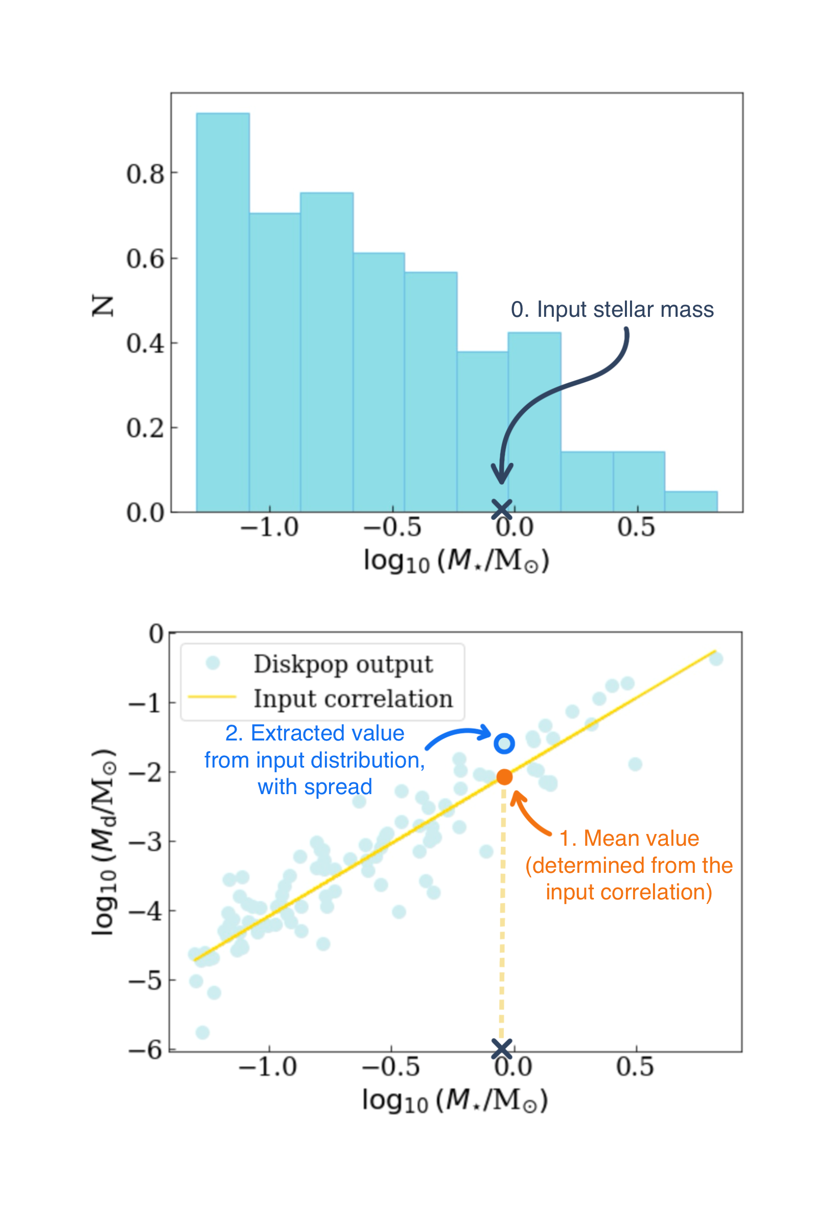
Representative sketch to show the determination of the disc parameters (disc mass in this example) based on the correlations with the stellar mass.
3.2. Evolution algorithm
Once the initial population is generated, its evolution proceeds depending on the chosen prescription. When possible, Diskpop gives the option to evolve the population analytically: as the evolution is muh faster using analytical prescriptions, this option should be preferred when available. However, some set ups do not allow for an analytical solution (for example, when internal photoevaporation is included) and there is therefore also th possibility to integrate the disc evolution equation numerically. In the following, we present the available analytical solutions, as well as the numerical integration algorithm.
3.2.1. Analytical solutions
In the following, we describe the three analytical solutions availale in Diskpop, divided by accretion model.
Viscous accretion
Self-similar solution: one of the most popular analytical solutions to the disc evolution equation (1) in the purely viscous case is the self-similar solution by Lynden-Bell & Pringle (1974), obtained assuming viscosity to scale as a power-law of the radius (\(\nu \propto R^{\gamma}\)).
The solution reads
and the disc mass and accretion rates as a function of time are given by
where \(\eta = (5/2 - \gamma)/(2 - \gamma)\) and the viscous timescale \(t_{\nu} = {R_c}^2/[3(2-\gamma)^2 \nu(R = R_c)]\) at the characteristic radius \(R_c\).
MHD wind-driven accretion
There are two classes of analytical solutions to Equation (1) in the MHD wind-driven scenario, associated with a specific prescription of \(\alpha_{\mathrm{DW}}\) (Tabone et al. 2022).
The simplest class of solutions (so-called hybrid solutions), which highlight the main features of wind-driven accretion in comparison to the viscous model, assume a constant \(\alpha_{\mathrm{DW}}\) with time; these solutions depend on the value of \(\psi \equiv \alpha_{\mathrm{DW}}/\alpha_{\mathrm{SS}}\), which quantifies the relative strength of the radial and vertical torque. In this case, the solution reads
and the disc mass and accretion rate will be
where \(\dot{M}_0\) is defined as \(\dot{M}_0 = \frac{\psi + 1 + 2 \xi}{\psi + 1} \frac{M_0}{2 t_{\mathrm{acc}, 0}} \frac{1}{(1+f_{\mathrm{M}_0})}\) and the other parameters are described in disc evolution.
Another class of solutions, which describe the unknown evolution of the magnetic field strength, assume a varying \(\alpha_{\mathrm{DW}}\) with time. To obtain these, (Tabone et al. 2022) parameterised \(\alpha_{\mathrm{DW}}(t) \propto \Sigma_{\mathrm{c}} (t)^{-\omega}\), with \(\Sigma_{\mathrm{c}} = M_{\mathrm{d}}(t)/2 \pi {R_c}^2 (t)\) (where \(R_c\) is a characteristic radius) and \(\omega\) as a free parameter, and neglect the radial transport of angular momentum (\(\alpha_{\mathrm{SS}} = 0\)). The solution in this framework reads
and the disc mass and accretion rate are
3.2.2. Numerical integration
Our solution algorithm employs an operator splitting method: the original equation is separated into different parts over a time step, and the solution to each part is computed separately. Then, all the solutions are combined together to form a solution to the original equation. We split Equation (1) into five different pieces, related to viscosity, wind-driven accretion onto the central star, wind-driven mass loss, internal and external photoevaporation respectively. Furthermore, Diskpop includes the possibility to trace the dust evolution in the disc, which is split in radial drift and dust diffusion. In the following, we describe the solution algorithm for each process.
Viscous accretion: the standard viscous solver is based on the freely available code by Booth et al. (2017). We assume a radial temperature profile \(T \propto R^{-1/2}\), which results in \(c_{s} \propto R^{-1/4}\) and \(H/R \propto R^{1/4}\). Note that this implies \(\nu \propto R\) (i.e., \(\gamma = 1\)). We assume \(H/R = 1/30\) at 1 AU and a mean molecular weight of 2.4. We refer to the original paper for details on the algorithm.
Wind-driven accretion: the second term in Equation (1) is effectively an advection term. The general form of the advection equation for a quantity q with velocity v is \(\partial_t q(x, t) + v \partial_x q(x, t) = 0\); in the case of wind-driven accretion, the advected quantity is \(R \Sigma\), while the advection (inwards) velocity is given by \(v_{\mathrm{DW}} = (3 \alpha_{\mathrm{DW}} H c_s)/2R\). We solve the advection equation with an explicit upwind algorithm (used also for dust radial drift).
Wind-driven mass loss: the mass loss term (third in Equation (1)) does not involve any partial derivative, and therefore is simply integrated in time multiplying by the time step.
Internal photoevaporation: effectively, internal photoevaporation (implemented through the model of Owen et al. 2012) is another mass loss term - therefore, as above, its contribution is computed with a simple multiplication by the time step. Once the accretion rate of the disc drops below the photoevaporative mass loss rate, a gap opens in the disc at the radius of influence of photoevaporation: in the model of Owen et al. (2012), the prescription changes depending on the radial location in the disc, with respect to the gap itself. Later, the gap continues to widen; when it eventually becomes larger than the disc, we stop the evolution and consider the disc as dispersed.
External photoevaporation: for a given stellar mass and FUV flux experienced by the disc, the mass loss rate arising from external photoevaporation is obtained, at each radial position, from a bi-linear interpolation of the FRIEDv2 grid (Haworth et al. 2023) using the disc surface density at each radial cell. The outside-in depletion of material is implemented following the numerical approach of Sellek et al. (2020): we define the _truncation_ radius, \(R_{\mathrm{t}}\), as the position in the disc corresponding to the maximum photoevaporation rate (which is related to the optically thin/thick transition of the wind), and we remove material from each grid cell at \(R>R_{\mathrm{t}}\) weighting on the total mass outside this radius. The mass loss attributed to the cell i can be written as:
\[\dot{M}_{\mathrm{ext},i} = \dot{M}_{\mathrm{tot}} \frac{M_{i}}{M(R>R_{\mathrm{t}})},\]where \(M_{i}\) is the mass contained in the cell \(i\), and \(\dot{M}_{\mathrm{tot}}\) is the total mass loss rate outside the truncation radius.
Dust evolution: based on the two populations model by Birnstiel et al. (2012) and the implementation of Booth et al. (2017). We consider the dust grain distribution to be described by two representative sizes, a constant monomer size and a time-dependent larger size, which can grow up to the limit imposed by the fragmentation and radial drift barriers. We evolve the dust fraction of both sizes following Laibe&Price (2014), and also include a diffusive term: the diffusion comes from the coupling with the turbulent gas, which has the effect of mixing the dust grains, counteracting gradients in concentration (Birnstiel et al. 2010). The dust-gas relative velocities are computed following Tanaka et al. (2005) and include feedback on the gas component. We refer to Booth et al. (2017) for details on the numerical implementation.
The separate pieces of Equation (1) must be solved over the same time step to be joined in a coherent solution. We calculate the time step for each process imposing the Courant-Friedrichs-Lewy (CFL) condition. The CFL condition reads \(\Delta t = C \mathrm{ min}(\Delta x / v)\) and ensures that, within one time step \(\Delta t\), the material moving at velocity _v_ does not flow further than one grid spacing \(\Delta x\). The Courant number _C_ must be positive and smaller than 1, with \(C = 1\) corresponding to the maximum allowed timestep to keep the algorithm stable. In our implementation, we pick \(C = 0.5\). We use zero gradients boundary conditions, setting the value of the first and last cell in our grid to that of the second and second to last. We solve the equation on a radial grid of \(10^3\) points with power-law spacing and exponent \(1/2\), extending from \(3 \times 10^{-3}`\) au to \(10^4\) au. From the physical point of view, this choice corresponds to assuming boundary layer accretion (see., e.g., Popham et al. 1993, Kley&Lin 1996) - however the difference from magnetic truncation accretion is negligible beyond \(\sim 10^{-3}\) au.
After each process has been solved separately, all the pieces are put back together to compute the new surface density, from which the integrated disc quantities are then calculated. As each disc evolves independently of the others in the population, the solver can easily be run in parallel.
3.3. Disc dispersal
In Section 1, under disc dispersal, we have discussed the physical mechanisms that can lead to the dispersion of protoplanetary discs. From the numerical point of view, disc in Diskpop are considered dispersed if they satisfy one of two conditions:
Reaching an input mass threshold. To account for the observational limits in detecting very low-mass discs, the _limit_discmass_ parameter in parameters.json can be set to represent the lowest possible disc gas mass after which the disc will be considered as effectively dispersed. This also allows to analyse the impact of more or less conservative assumptions on the observational sensitivities. When this condition is reached, the code prints on screen “Disc with identifier # has been dispersed!”.
Internal photoevaporation carving too large of a gap. When internal photoevaporation is present, a gap opens within the disc and grows in time. Eventually, the gap might become larger than the disc itself: in that case, the disc is effectively dispersed, and the code will print on screen “The hole is too large - I will stop the evolution now”.
Once a disc is dispersed, it moves from being a Class II object to a Class III (a discless star) and keeps on evolving while only updating the stellar parameters.